- Jul 2, 2021
- 12 min read
Written By
- Vincent Stettler
This is joint work with Julien Herzen. The complete code is available here.
In this post, we reverse the direction of traditional machine learning. Usually the direction is from data to a property: One builds a model that predicts for a data point a certain property. We are going to explore the other direction: from property to data point. Our high-level goal is to start with a desired property, and to modify a data point until that property is satisfied.
Consider the toy dataset MNIST, where the usual goal is to build a classifier that takes as input an image of a handwritten digit and predicts the digit that is being depicted. This prediction can be understood as a likelihood vector that assigns a certain probability to each possible digit. In the figure below, we see that the classifier assigns the highest probability to the digit 7.
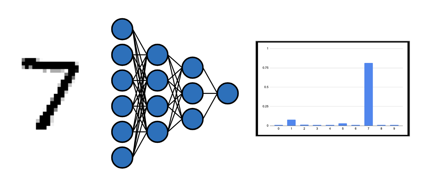
A neural network classifier that predicts the digit being depicted in the input image.
We reverse the direction and ask if we can impose another likelihood vector, for example, one where the digit 3 is the most likely, and modify the original image such that it indeed depicts the digit 3. We will take an approach that is fairly generic, and that, when it works, will prove powerful because it will allow us to generate new samples that have desired properties.
We refer to this kind of optimization as ‘model-based optimization’. We will focus on a gradient-based technique where we use the gradient of models to navigate the latent space of a Variational Auto-encoder with the intention to optimize certain properties. As an example, we will gradually build a solution that lets us change the digit that is being depicted in an image, or lets us increase the thickness of the stroke of the digit.
First, we will discuss (gradient-based) model-based optimization in more details. Then we will elaborate on the reason why we perform the optimization in the latent space of a VAE, and finally we discuss the method, present the PyTorch implementation, and show the results.
Model-Based Optimization Using Gradients
On an abstract level, we are interested in optimizing certain properties of data points by altering them. The method we are going to describe is general in a sense that it — in theory — works for any type of data and any property. In this article we are working with MNIST images and aim to increase their thickness and to change the digit being depicted.
By model-based optimization we mean that we do not directly optimize the property itself, but instead we optimize the output of a model of that property. Often, there are situations where the property that is to be optimized is not accessible in a closed form, so direct optimization is not tractable. For such properties it therefore makes sense to first build a (good) predictive model and then to optimize the prediction of that model.
We focus on gradient-based optimization and therefore require that the models are differentiable. For the following discussion we assume that we have a good model that predicts the thickness of a MNIST image. The gradient of the model output (thickness) with respect to the model input (image) is a vector that points to the local direction in the space of images where the thickness increases most. So if we have an image, we can compute the gradient of the model with respect to the image, and then alter the image a little bit into the direction of the gradient. By doing so, we effectively increase (by a small amount) the predicted thickness for the image. Mathematically speaking, we are doing the following:

Equation (1): The equation that describes one optimization step. x0 is the image, T̂ is the thickness prediction model, and η is the amount by which we alter the image (step size).
Since the gradient only locally points into the desired direction, we cannot simply increase the step size and hope to increase the thickness more. This would lead to an overshoot. What we do instead, is to apply the above alteration iteratively, always re-computing the gradient after each step. This really is the same gradient descent process most of us are used to in order to tune neural networks’ parameters, except that here we apply it to the data instead of the parameters.
About Manifolds
Before we continue, we need to talk about data manifolds, and the distinction between them and the data space. The data space is the mathematical space that contains all data points. For MNIST images this would be the space of all 784-dimensional pixel vectors. The data manifold, on the other hand, is the sub-space that contains only “valid” MNIST images. The meaning of the term “valid” is a bit vague, and defining it could be a blogpost on its own. Let’s just say that a valid MNIST image is an image that shows a digit which looks like a real handwritten digit. The following image illustrates the concept further.
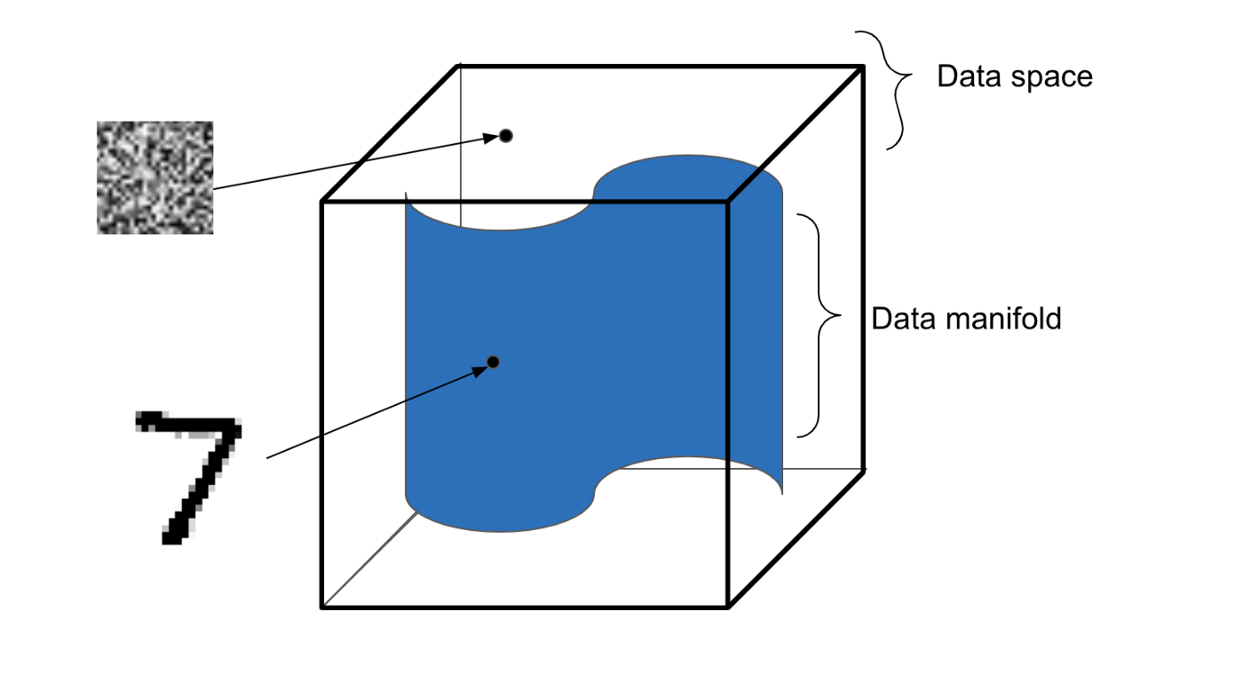
Illustration of distinction between the data space and the data manifold.
Usually, high dimensional data is distributed sparsely in the data space, and altering a data point has a high probability of producing a data point that is outside the manifold, e.g., does not look like a real image of a digit.
In order to show this, we trained a digit classifier with an accuracy of 98%. Then, we took an original image of a 7 and applied the iterative optimization described in Equation (1), directly on the data space. Our goal was to gradually transform the image of a 7 into an image of a 2, by maximising the corresponding output of the model.
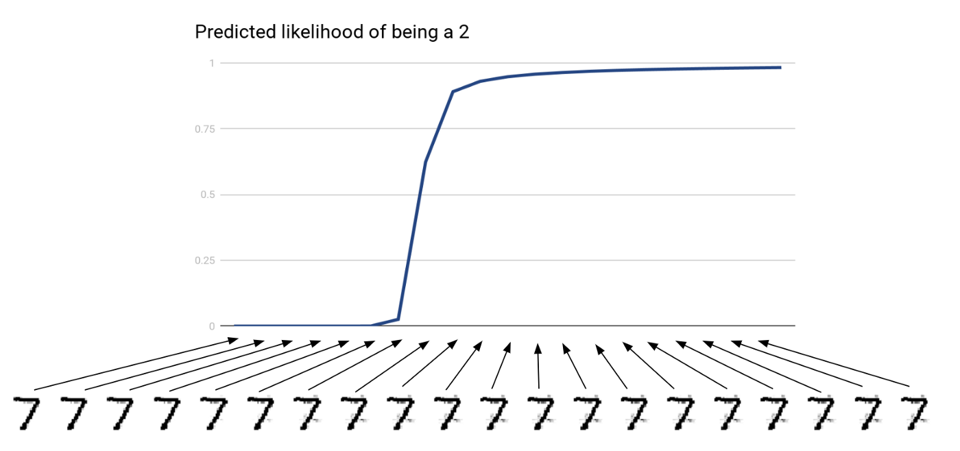
Result of optimizing directly in data space. The x-axis corresponds to successive optimization steps and the y-axis shows the predicted likelihood of the image being a 2.
We see that the experiment was both successful (in the sense that the resulting image indeed is predicted as being a 2) and unsuccessful (in the sense that the resulting image does not actually look like a 2). As mentioned above, the optimization in data space has too much freedom and nothing prevents it from leaving the data manifold. Here we see that the optimization procedure went outside of the manifold, because the later images show unnatural artifacts on the image which could not have been originated from a drawing stroke.
During the training, the classifier only gets to see images from within the data manifold. However, the classifier predicts somethingfor any possible data point in the data space. Therefore, the optimization can leave the manifold and find a region where the model predicts the desired digit. We observe that the optimization does not even need to go far, as the images still do look a lot like the original image. The reason for this that neural networks are very vulnerable to what is called adversarial perturbations. This, however, is beyond the scope of this article and we refer to this post for more information about this.
In order to prevent this we have to make sure that we only alter the data points along the manifold. This would mean that we restrict our optimization to the data manifold, such that we produce only valid images of digits. One way of doing this is to use manifold learning.
(Variational) Auto-encoders And Manifold Learning
Auto-encoders are a special type of neural network used (among other things) for manifold learning. Using an encoder-decoder architecture with a low-dimensional code space in-between, they are trained to minimize the difference between the input and output. Because of the low dimensionality of the code space there is an information bottleneck effect that forces the auto-encoder to learn a meaningful, low-dimensional representation of the data space (i.e., the manifold). The following image illustrates the architecture of an auto-encoder. On the left side we see the inputs, real MNIST images, and on the right side we see their reconstructions.
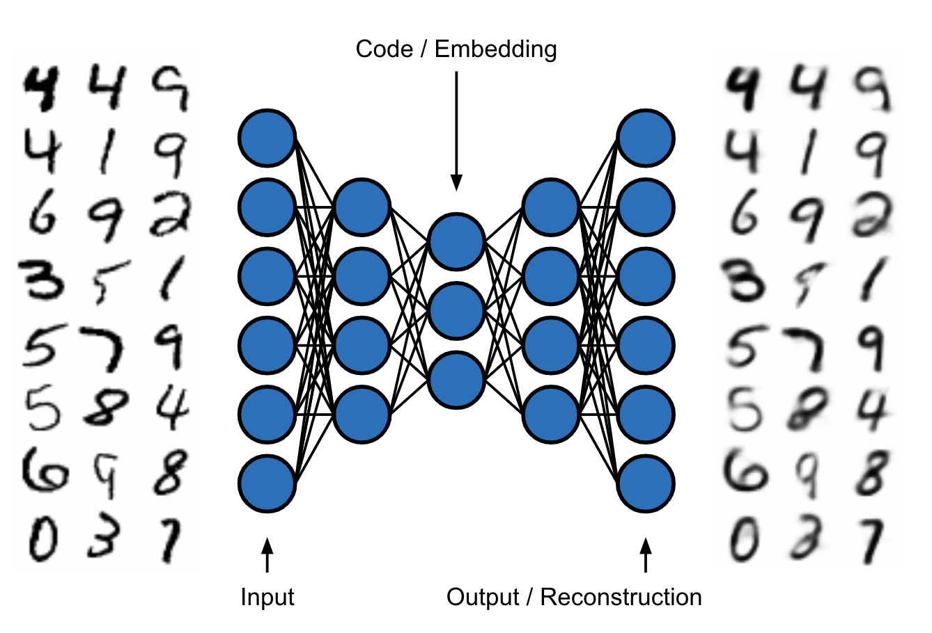
Illustration of an auto-encoder.
Recall that our previous problem was that the optimization has too much freedom when applied directly in the data space. Now, assuming that we trained such an auto-encoder, we can apply the optimization in the low-dimensional code space instead (i.e., “force” the optimization to stay on the manifold). The next image shows the distribution of the code points of real MNIST images in the two-dimensional code space of an auto-encoder.
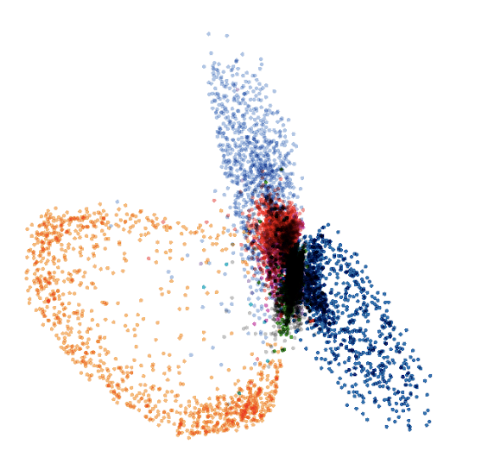
Code space distribution of MNIST in an auto-encoder. Different colors correspond to different labels.
We observe that the code space distribution is unfortunately not very compact. This is a well-known property of vanilla auto-encoders: They tend to produce a fractured code space distribution, meaning that there are “holes” in the code space with low probability mass. The optimization might then guide the code point into such a region where the decoder was never trained on. We see this for example between the orange (corresponding to the digit 1) and the light blue (digit 5) clusters. If we wanted to change an image of a 1 into an image of a 5, then the optimization might guide us into the unknown, away from the manifold. This could potentially lead to the same problem we encountered previously.
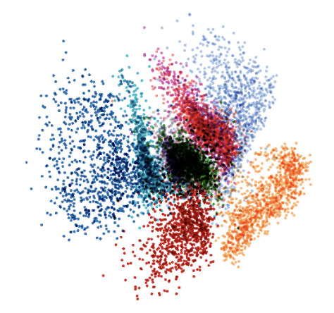
Code space distribution of MNIST in a variational auto-encoder. Different colors correspond to different labels.
For this reason we do not use vanilla auto-encoders but Variational Auto-encoders. Simplistically speaking, they are vanilla auto-encoders trained with an additional loss term (Kullback–Leibler divergence) that pulls the code distribution into the direction of a standard normal distribution. This has the effect that the code points are distributed in a smoother way, decreasing the probability that the optimization moves the code point into a low-density region.
Multi-Head Training
So to summarise, we train a Variational Auto-encoder to unlock the ability to restrict the optimization to the data manifold. This means that we perform the optimization on code points before we decode the final (optimized) code point back into data space.
This gives us two possibilities for the predictive model. Either we train the model on top of the data space (i.e. it takes decoded code points as input), or directly on top of the code space. In this article we explore the second option for two reasons. First, if the model would take as input points in data space we would have to decode the code points first before feeding them into the model. Since the decoder itself is not perfect, this would introduce an additional source of error. Second, if the model works on the code space directly, then we can train it simultaneously with the Variational Auto-encoder. This simultaneous training means that the encoder not only is trained to produce code points that can be decoded with a low reconstruction error, but also to encode information that is relevant for the predictive model. This means that the code space can get semantically shaped according to the property that is to be optimized. The following figure illustrates the architecture of the our model.
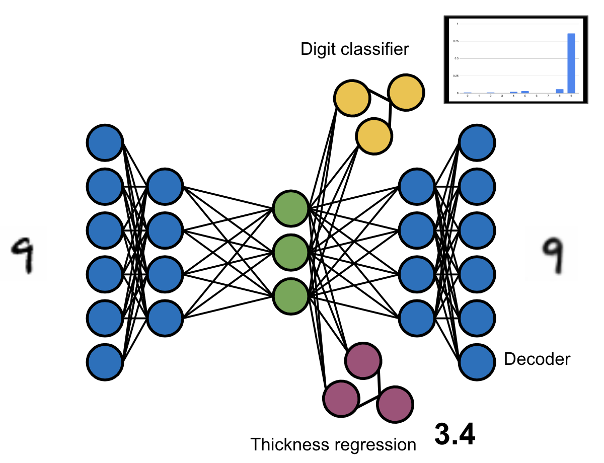
Conceptual depiction of the architecture of our multi-head variational auto-encoder. The blue circles corresponds to the encoder and decoder, the green ones to the code space, the yellow ones to the digit classifier, and the purple ones to the thickness prediction.
We train a Variational Auto-encoder with two predictive models: A thickness regression and a digit classification model. The following code snippet shows our code for this model.
We define a PyTorch module VAE which contains four sub-modules: the encoder, the decoder, and the two predictive models classifier and thickness_model. For each head of the model we use different loss functions and metrics, corresponding to the task that is performed by the head. The total loss is the simple sum of all the individual losses and the KL-divergence. Note that more sophisticated implementations might use a weighted sum instead. The encoder and decoder modules contain convolutional layers as well as fully-connected layers. The two predictive models are fully-connected neural networks. The full code and architectures can be found here.
Training the digit classifier is easy because the dataset already contains the corresponding labels. This is unfortunately not the case with the thickness labels. Therefore, we need to first compute the ground truth thickness of the MNIST images. Fortunately, the paper Morpho-MNIST: Quantitative Assessment and Diagnostics for Representation Learning describes how to do this in detail. Our implementation follows their approach and applies the following steps to each image. First, we upscale and binarize the image. Then we apply the euclidean distance transform and compute the skeleton. The distance map stores for each pixel the distance to the border of the digit. The thickness is then simply twice the mean of the distance map over every pixel in the skeleton. The library skimage offers easy-to-use implementations of algorithms like the euclidean distance transform.
Let’s Increase The Thickness!
Now we can finally apply the optimization. As mentioned previously we want to iteratively modify a code point in a direction that increases the thickness of the corresponding data point. We do this by first computing the gradient of the thickness prediction with respect to the code point and evaluate it at our current code point. This gradient points into the direction of steepest descent. In other words, it points into the direction in which the thickness (as predicted by our model) increases the most. After following the gradient for some steps the code point hopefully corresponds to a higher thickness than the point we started from.
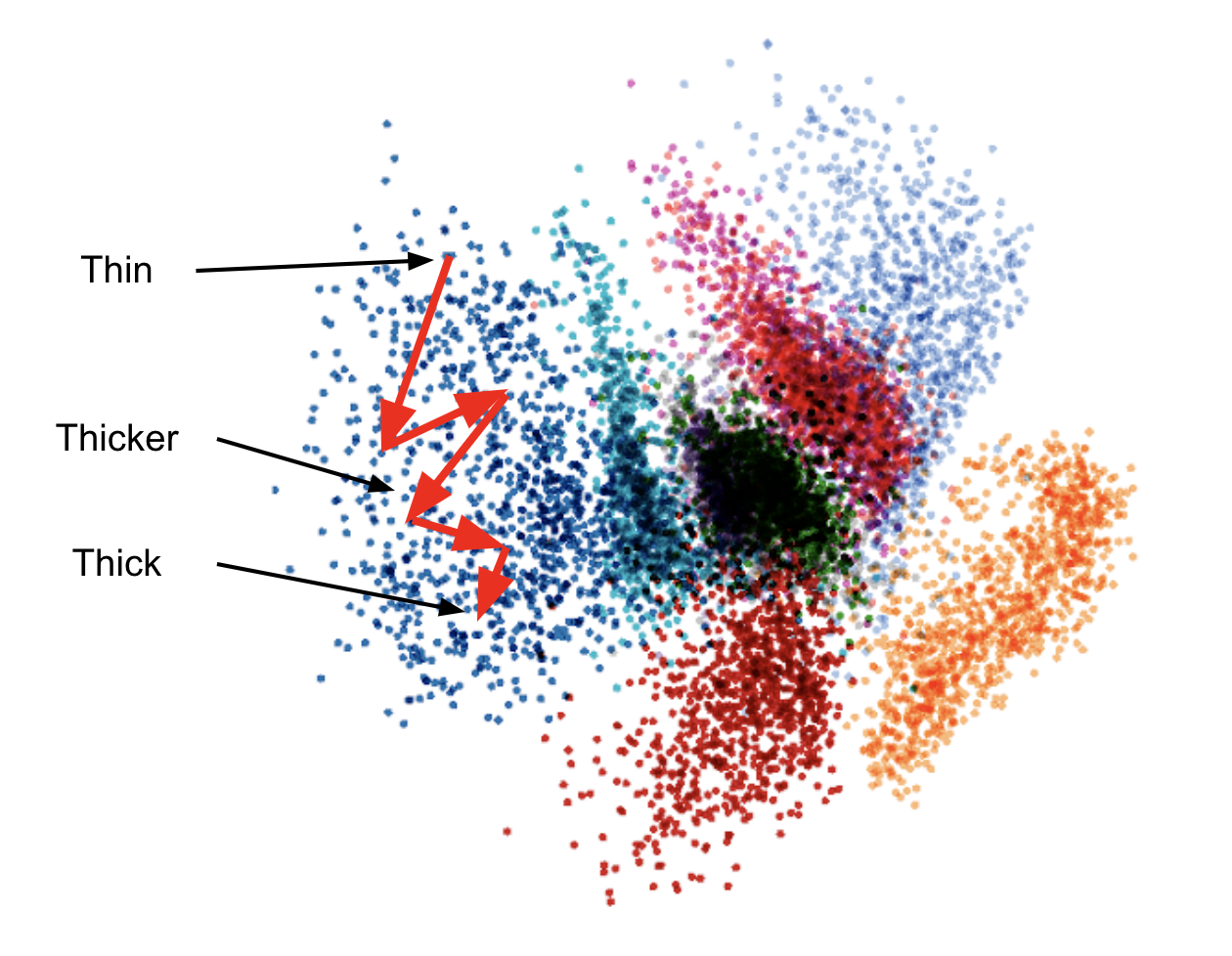
Illustration of the model-based optimization in the code space of a variational auto-encoder. The red arrows show the iterative optimization that increases the thickness of the corresponding image.
The following code snippet shows the code to perform the optimization. After having computed the prediction of the thickness, we call backward on the prediction to compute the gradient. The variable z denotes the code point, and the gradient with respect to the code point can then be found with z.grad.
The following image shows each step of such an optimization, where we start off from a random (standard normal) code point of dimensionality 16. We see that our experiment worked, the thickness does increase! Furthermore, observe how the digit and the style (apart from the thickness of course) stays the same. This is not trivially true, because the optimization procedure does not explicitly try to conserve the digit or the style.

Model-based thickness increase
Changing Digits
We did not train two predictive heads for no reason: Now we want to play with the digit classifier. Our goal is to take the same random (standard normal) point as above and gradually change it into another digit. For this we want to use our optimization to increase the prediction of the image being a certain digit. For the digit i we compute the gradient of the i-th output of the classifier and iteratively step into this direction. The following image shows the result of exactly that. It works !
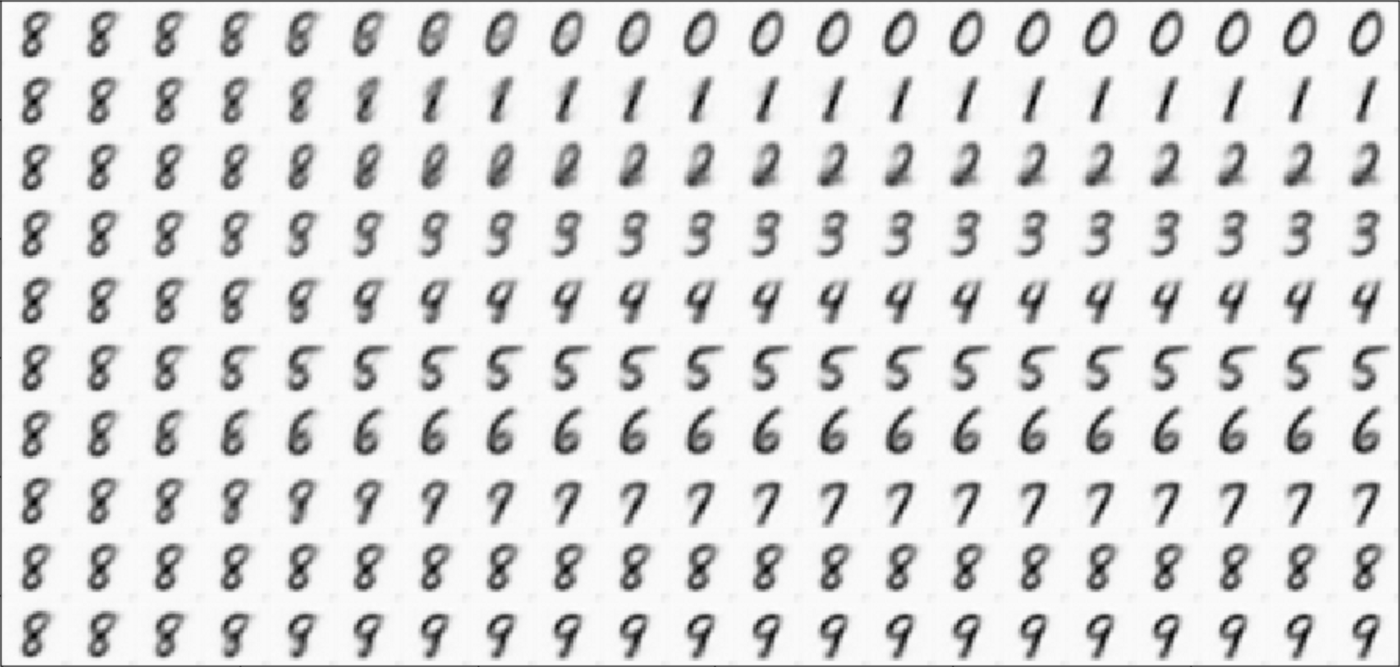
Model-based digit change
Possible Improvements
This is only a basic implementation and there is obviously a lot to improve. Instead of doing a fixed number of steps, one could think about other termination criteria, like for example stopping if the gradient gets close to zero. One might also be interested in multi-criteria model based optimization, where the idea would be to optimize multiple properties of a data point. In such cases, it is possible for instance to follow weighted sums of the gradients of the respective models.
Moreover, our basic implementation “blindly” applies the gradient updates, being in danger of leaving the data manifold. Even though we did not encounter this problem in our experiments, it might very well happen with a more complex dataset. In a more sophisticated implementation one might therefore employ measures to guarantee that this does not happen, such as making sure the gradient ascent procedure does not navigate the latent space too far off from any point on the data manifold.
Conclusion and Business Applications
In this post we explored the topic of model-based optimization and we have seen how to use the gradient of a model to navigate the latent space of a variational auto-encoder. We ended up with a model that can be used to make MNIST images more thick, or to change one digit into another.
The data we used consisted of simple images for the purpose of illustrating how the approach works using visual support. However, the method is much more general and can be applied to a variety of interesting domains. Here are two examples of business applications of the method described:
Instead of optimizing images we can optimize molecules. If we can predict the effectiveness in treating a certain disease, then we can optimize and discover molecules that can be used as a drug for that disease. But we might even go a step further and do multi-criteria optimisation, where we additionally minimize some non-desirable side-effects of the drug.
Another area where the method could be applied is writing, for example in the field of text enhancement or text simplification. A possible approach would be to build a model that predicts the eloquence of a text. Then one could use this model in order to increase the quality of texts.
In summary, the method does not come short when it comes to applicability. Maybe even your data can be optimised — if you are interested in discussing your use-case or idea, please get in touch with us.
Thanks to Julien Herzen and Rudolf Höhn.
