
- Jul 6, 2021
- 11 min read
- Julien Herzen
Any quantity varying over time can be represented as a time series: sales numbers, rainfalls, stock prices, CO2 emissions, Internet clicks, network traffic, etc. Time series forecasting — the ability to predict the future evolution of time series— is thus a key capability in many domains where anticipation is important. Until recently, the most popular time series forecasting techniques were focusing on isolated time series; that is, predicting the future of one time series considering the history of this series alone. Since a couple of years, deep learning has made its entry into the domain of time series forecasting, and it’s bringing many exciting innovations. First, it allows for building more accurate models that can potentially capture more patterns and also work on multi-dimensional time series. Second, these models can also potentially be trained on multiple related series. There are many contexts where this capability can be beneficial: for instance for electricity producers observing the energy demand of many of their customers, or for retailers observing the sales of many potentially-related products. However, one commonly-occurring drawback is that such deep learning models are typically less trivial to work with for data scientists than some of their simpler statistical counter-parts. That is, until Darts came around 🙂
One of the missions of the open-source Darts Python library is to break this barrier of entry, and provide an easy and unified way to work with different kinds of forecasting models.
In this post, we’ll show how Darts can be used to easily train state-of-the-art deep learning forecasting models on multiple and potentially multi-dimensional time series, in only a few lines of code.
A notebook containing code and explanations related to this article is available here. If you are new to Darts, we recommend to start by reading our earlier short introductory blog post.
Create a Global Forecasting Model
from darts.models import RNNModel

model = RNNModel(...hyper_parameters...)
Models working with multiple time series are:RNNModel, BlockRNNModel, TCNModel, NBEATSModel, TransformerModel and RegressionModel (incl. LinearRegressionModel and RandomForest).
Train a Model on Multiple Time Series
model.fit([series1, series2, …])
Forecast Future Values of Any Series
future = model.predict(n=36, series=series_to_forecast)
Train and Forecast with Past and/or Future Covariates Series
model.fit(series=[series1, series2, ...],
          past_covariates=[past_cov1, past_cov2, ...],
          future_covariates=[future_cov1, future_cov2, ...])

future = model.predict(n=36,
                       series=series_to_forecast,
                       past_covariates=past_covariate_series,
                       future_covariates=future_covariate_series)
future_covariates have to be known n time steps in advance at prediction time.
Training a Model on Multiple Series
All the deep learning forecasting models implemented in Darts as well as RegressionModel are global forecasting models. This means that these models can be trained on multiple series, and can forecast future values of any time series, even series that are not contained in the training set. In contrast, the other non neural-net forecasting models in Darts (ARIMA, Exponential Smoothing, FFT, etc) are currently all local models — namely, they are trained on a single time series to forecast the future of this series.
The ability to train a single model on multiple series is a very important feature, because usually deep learning models shine most when they are trained on an extensive amount of data. It allows them to match patterns across a potentially large amount of related time series. For example, the N-BEATS model published recently obtains wining forecasting performance when trained on tens of thousands of time series in the M4 competition (a well-known forecasting competition). We have implemented N-BEATS in Darts, and so it can now be trained and used out-of-the-box on large datasets with only a few lines of code.
In a future article, we’ll show an example of how to train such large models on big datasets. For the time being however, we would like to expose the functionalities and mechanics of global models in Darts, from the point of view of users who need to understand and control what’s going on.
Predicting Air Traffic Using Cow Milk Production…
As a toy/cartoon example, we’ll train a model on two time series that have not much in common. Our first series contains the number of monthly airline passengers in the 1950’s, and our second series contains the monthly milk production (in pounds per cow) around the 1960’s. These two series obviously represent two very different things, and they do not even overlap in time. However, coincidentally, they express quantities in similar orders of magnitude, so we can plot them together:
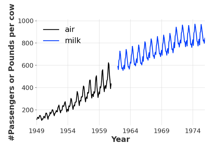
Monthly number of air passengers and monthly milk production per cow (in pounds)
Although different, these series share two important characteristics: a strong yearly seasonality, and an upward trend, which could perhaps be seen as an effect of the general economic growth of this era (from looking at the blue curve we can ask ourselves whether cows’ overall well-being has also been on an upward trend; but that’s a different topic).
Training on Multiple Series
Training a model on several series (in this case two) is really easy with Darts, it can be done like that:
from darts.models import NBEATSModel
model_air_milk = NBEATSModel(input_chunk_length=24,
                             output_chunk_length=12)
model_air_milk.fit([train_air, train_milk])
In this code snippet, we create an NBEATSModel instance (we could also have used any other global model). The input_chunk_length and output_chunk_length parameters specify the lengths of the time series slices taken by the internal N-BEATS neural network in input and output. In this case, the internal neural net will look 24 months in the past and produce forecasts by outputting “chunks” of 12 points in the future. We’ll give more details on these parameters later.
We then train our model by calling the fit() method with a list of series to train on. Here, train_air and train_milk are two TimeSeries instances containing the training parts of the series.
Producing Forecasts
Once the model is trained, producing forecasts for one (or several) series is a one-liner. For instance, to forecast the future air traffic, we would do:
pred = model_air_milk.predict(n=36, series=train_air)
Note here that we can specify a horizon value n larger than the output_chunk_length : when this happens, the internal neural network will simply be called on its own outputs in an auto-regressive fashion. As always, the output of the predict() function is itself a TimeSeries. We can quickly plot it, along with the prediction obtained when the same model is trained on the air series alone:
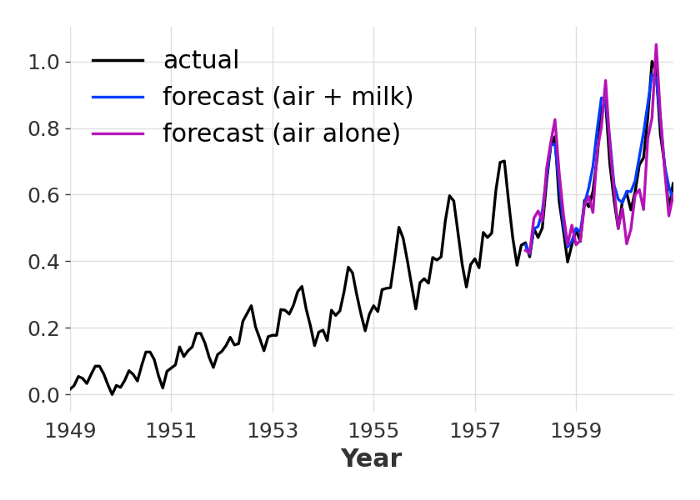
Two forecasting models for air traffic: one trained on two series and the other trained on one. The values are normalised between 0 and 1. Both models use the same default hyper-parameters, but the number of epochs has been increased in the second model to make the number of mini-batches match.
In this case we get a MAPE error of 5.72% when the model is trained on both series, compared to 9.45% when trained on the air passengers series alone.
Well, that’s an important question, no doubt. And in this very particular case, for this particular set of model and data, it seems to be the case. This is not so surprising though, because here the model just gets more examples of what monthly time series often look like. We can think of the milk series as providing a sort of data augmentation to the air series. This obviously wouldn’t necessarily work for any combination of unrelated time series.
Producing Forecasts for Any New Series
Note that we can also just as easily produce forecasts for series that are not in the training set. For the sake of example, here’s how it looks on an arbitrary synthetic series made by adding a linear trend and a sine seasonality:
from darts.utils.timeseries_generation import linear_timeseries, sine_timeseries

series = 0.2 * sine_timeseries(length=45) +
linear_timeseries(length=45, end_value=0.5)

pred = model_air_milk.predict(n=36, series=series)
Even though our synthetic series has not much to do with either air traffic or milk (it doesn’t even have the same seasonality, and it has a daily frequency!), our model is actually able to produce a decent-looking forecast (note that it probably wouldn’t work well in most cases).
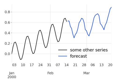
This hints to some pretty nice one-shot learning applications, and we’ll explore this further in future articles.
How it Works (Behind the Scenes)
It’s helpful to go slightly more in details and understand how the models work. You can skip this section if you’re not interested or if you don’t need more control.
Model Architecture
So how does it look internally? First, as already mentioned, the internal neural net is built to take some chunks of time series in input (of length input_chunk_length), and produce chunks of time series in output (of length output_chunk_length). Importantly, a TimeSeries in Darts can have several dimensions — when this happens the series is called multivariate, and its values at each time stamp are simply vectors instead of scalars. For example, the inputs and outputs on a model working with “past covariates” look like this:
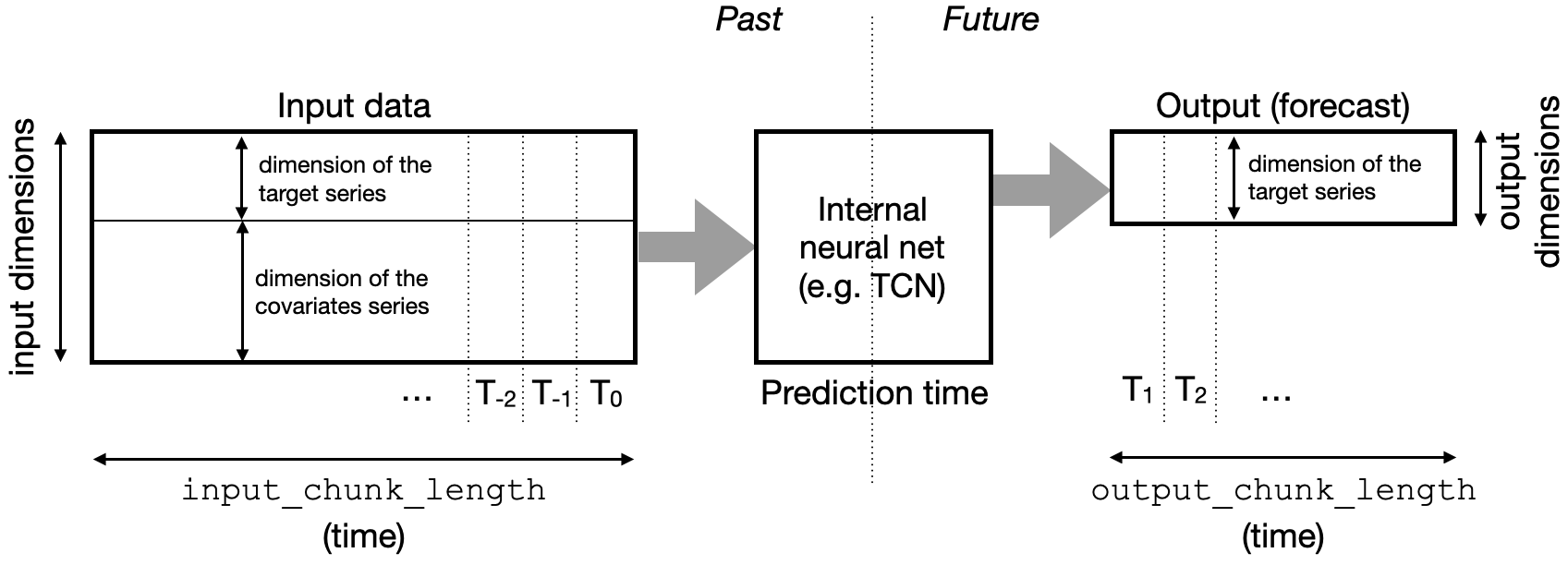
The input and output time series chunks consumed and produced by the neural network to make forecasts. This example is for “past covariates” model; where past values of the covariate series are stacked with past target values to form the neural net input.
We distinguish two different kinds of time series: the target series is the series we are interested to forecast (given its history), and optionally some covariate series are other time series that we are not interested to forecast, but which can potentially help forecasting the target. Both target and covariate series may or may not be multivariate — Darts will automatically figure out the right input/output dimensions of the internal neural net based on the training data. In addition, some models support “past” covariates — i.e. covariate series whose past values are known at prediction time, while others support “future” covariates — i.e. covariate series whose future (and possibly historic) values are known at prediction time. These covariates are stacked with the target (their dimensions concatenated) in order to build the neural net input. We refer to this article for more information on past and future covariates in Darts.
Finally, not all models need an output_chunk_length. RNNModel is a “truly recurrent” RNN implementation, and so it always produces outputs of length 1, which are used auto-recursively to produce forecasts for a desired horizon n. Our implementation of RNNModel is similar to DeepAR, and it supports future covariates.
Training Procedure
In order to train the neural network, Darts will build a dataset consisting of multiple input/output pairs from the provided time series. The inputs are used as inputs of the neural network and the outputs serve to compute the training loss. There are several possible ways to slice series to produce training samples, and Darts contains a few datasets in the darts.utils.data submodule.
By default, most models will use a SequentialDataset, which simply builds all the consecutive pairs of input/output sub-series (of lengths input_chunk_length and output_chunk_length) existing in the series. On two time series, the slicing would look as follows:
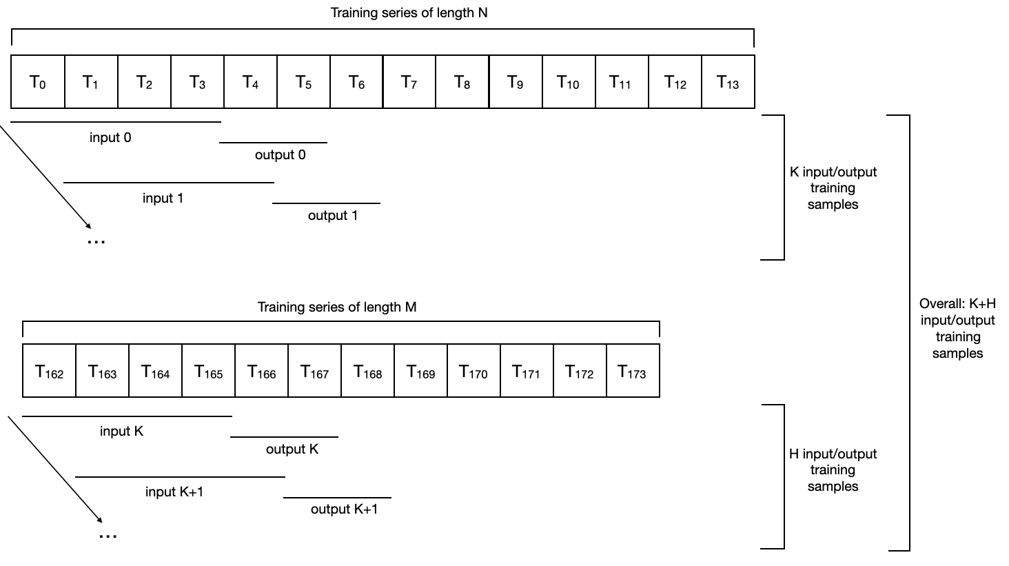
The slicing of two target time series to produce some input/output training samples, in the case of a SequentialDataset (no covariate in this example).
The series used for training need not be the same length (in fact, they don’t even need to have the same frequency).
As another example, HorizonBasedDataset is inspired from the N-BEATS paper, and produces samples closer to the end of the series, possibly even ignoring the beginning of long series.
All of the slicing operations done in datasets are done efficiently, using Numpy views of the arrays underlying the time series, in order to optimize training speed (a GPU can be used as well). To support large datasets that do not fit in memory, the Darts training datasets can also be manually built from Sequence’s of TimeSeries, which make it possible to implement lazy data loading. In this case, the models can be fit by calling fit_from_dataset() instead of fit(). Finally, if you need to specify your own slicing logic, you can implement your own training dataset, by subclassing TrainingDataset.
Using Covariates
Covariates represent time series that are susceptible to provide information about the target series, but which we are not interested in forecasting. As an example, we will build a synthetic series by multiplying two sines:
series1 = sine_timeseries(length=400, value_frequency=0.08)
series2 = sine_timeseries(length=400, value_frequency=0.007)
target = series1 * series2
covariates = series2
This is what these series look like when plotted:
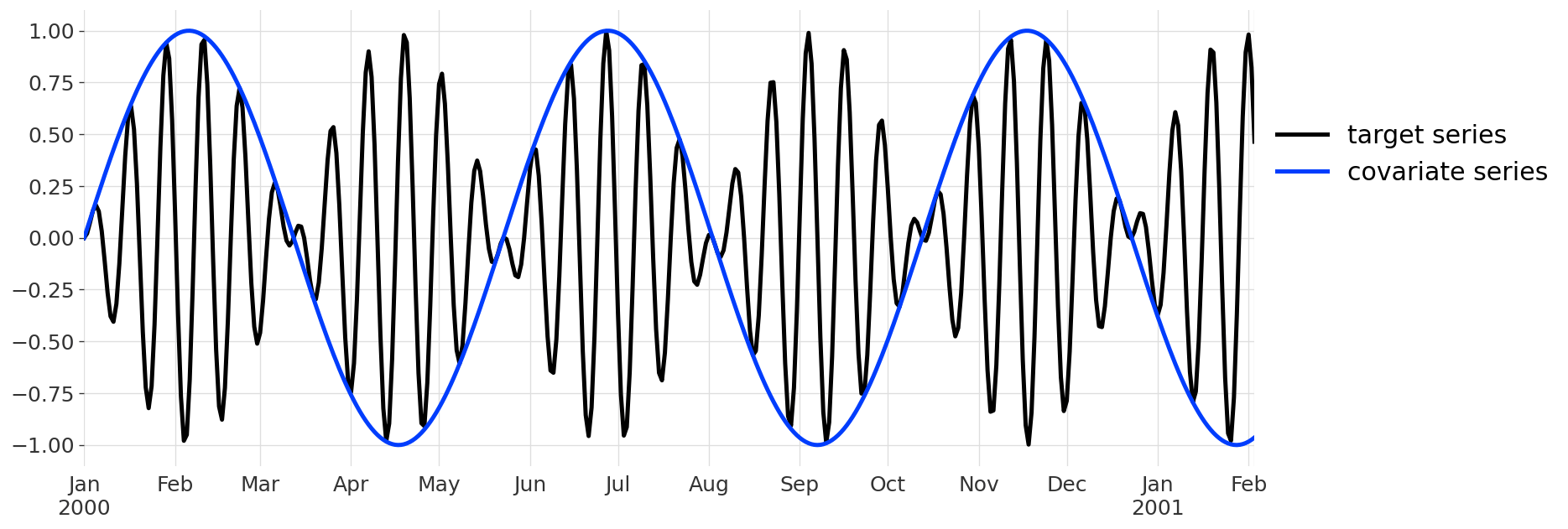
Let’s also split them in train and validation sub-series of lengths 300 and 100, respectively:
target_train, target_val = target[:300], target[300:]
cov_train, cov_val = covariates[:300], covariates[300:]
Let’s then build a BlockRNNModel model and fit it on the target series without using covariates:
from darts.models import BlockRNNModel

model_nocov = BlockRNNModel(input_chunk_length=100,
                            output_chunk_length=100,
                            n_epochs=200)

model_nocov.fit(target_train)
We can now get a forecast for 100 points after the end of the training series. As the series has many near-zero values, we’ll use the Mean Absolute Scaled Error to quantify the error:
from darts.metrics import mase

pred_nocov = model_nocov.predict(n=100)

mase_err_nocov = mase(target, pred_nocov, target_train)
Here’s what we get:
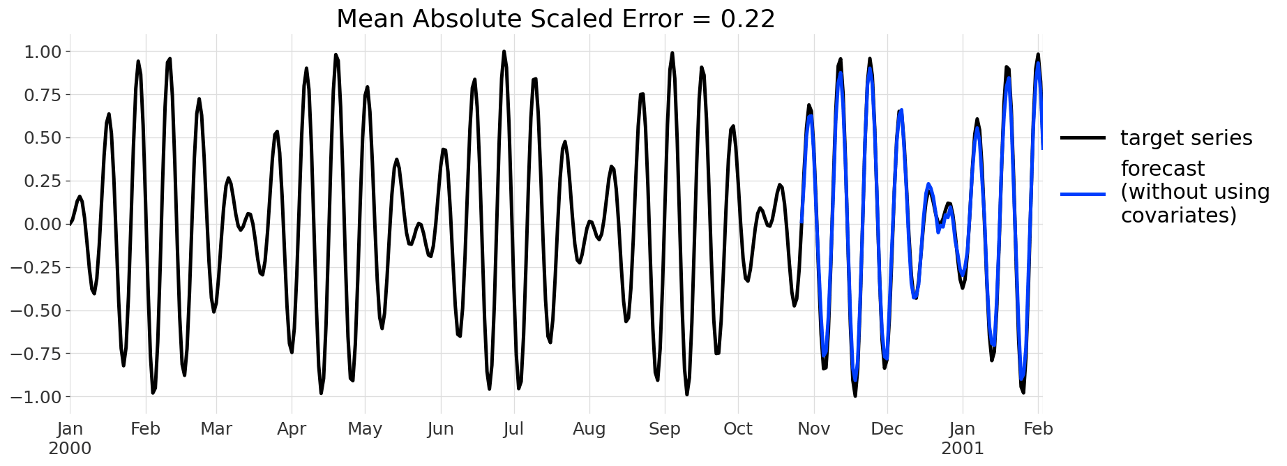
This is actually really not bad, given that we’ve just used a vanilla RNN with default parameters and we are producing a single 100-points ahead forecast. Let’s look if we can do even better by using the covariates series. Using covariates is meant to be really easy — we don’t even have to worry about it when building the model; we can just call fit() with a past_covariates argument specifying our past covariate series:
model_cov = BlockRNNModel(input_chunk_length=100,
                          output_chunk_length=100,
                          n_epochs=200)

model_cov.fit(target_train, past_covariates=cov_train)
The only difference (w.r.t. not using covariates) is that we specify past_covariates=cov_train when training the model. At prediction time, we also have to specify this past covariate:
pred_cov = model_cov.predict(n=100,
                             series=target_train,
                             past_covariates=cov_train)

mase_err_cov = mase(target, pred_cov, target_train)
And here’s the result:
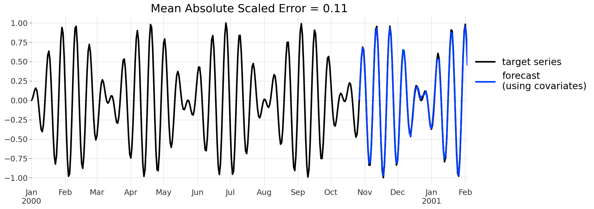
This forecast is even more spot-on than the previous one. In this case the covariate series explicitly informs the RNN about the slowly varying low frequency component of the target series. just by specifying the covariates, we’ve been able to divide the MASE error by 2, not bad!
Here we have used a BlockRNNModel, which supports past_covariates. Darts has other models supporting future_covariates, and we recommend checking this other article in order to have a better view of past and future covariates.
We have just seen in this example how to use covariates with models trained on a single target series. The procedure can however be seamlessly extended to multiple series. To do this, it’s enough to provide a list containing the same number of covariates to fit() and predict() as the number of target series. Let us also mention that backtesting (using either the backtest() or historical_forecasts() functions of models) and grid-searching hyper parameters (using the gridsearch() method) also support specifying past and/or future covariates.
Conclusions
We are very excited about the nascent success of applying deep learning to the domain of time series. With Darts, we are trying to make it extremely easy to train and use state-of-the-art deep learning forecasting models on a large number of time series. The latest release of Darts goes a long way in this direction, but we are still actively working on future developments, among which: a support for non- time-series conditioning and a treatment of probabilistic time series.
At Unit8, we are a team of software engineers and data scientists on a mission to democratise machine learning and good data practices in the industry, and we work on many other things besides time series. If you‘d like to talk with us, do not hesitate to get in touch.
Acknowledgements — We’d like to thank everyone who already contributed to Darts: Francesco Lässig, Léo Tafti, Marek Pasieka, Camila Williamson, and many other contributors. We’re always welcoming issues and pull requests on our github repo. You can also letting us know what you think by dropping us a line.
Thanks to Michal Rachtan, Gael Grosch, and Unit8.