Anomaly detection in healthcare data with Darts

Time series analysis in healthcare: overview

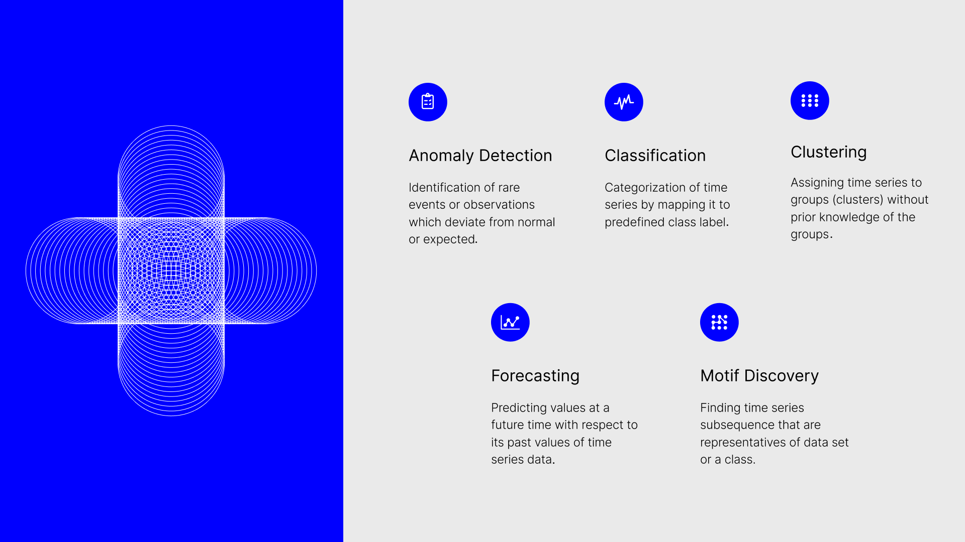
Time series methods play a crucial role in understanding temporal data in healthcare, allowing professionals to make informed decisions for improved patient outcomes, predictions, and patterns identification. They process information gathered chronologically through medical records including patient observations like vitals, hospital admission frequency, medicine dosages retrieved from sources like EHRs, registers, claims data, wearables, and additional healthcare data repositories. With this analysis, experts obtain valuable conclusions from intricate and multidimensional datasets. By exploiting time series examination to generate RWE regarding particular therapies, physicians gain knowledge critical to determining effective treatment plans while promoting overall patient welfare and optimizing health systems. Furthermore, considering the recurrent patterns in numerous health-related factors, like seasonal alterations and long-term tendencies, the application of time series scrutiny proves indispensable. Common applications of time-series analysis include:

• Anomaly detection: Identification of rare events/observations which deviate from the normal/expected.
  Example: detecting critical health episodes such as arrhythmia from electro-cardiogram (ECG) signals [1].
• Forecasting: Predicting future values for a time series with respect to its past values (and other external variables). Example: predicting the number of hospital patients to optimise resource allocation and staffing levels [2].
• Classification: Mapping time series to a class label.
  Example: predict patient risk categories based on historic time series data during COVID-19 pandemic [3].
• Clustering: Assigning time series to groups (clusters) without prior knowledge of the groups.
  Example: detect gene expression changes across single-cell RNA sequences [4].
• Motif Discovery: Finding time series subsequences that are representatives of a data set or a class.
  Example: differentiation between types of motifs in blood glucose levels to identify poor glycemic control (repeated glucose level spikes in a temporally located region) [5].

In this article, we are going to deep dive into the use case of anomaly detection, and showcase how to leverage our open-source library Darts for such type of analyses.

Anomaly detection in Darts

At Unit8, we’ve worked extensively on time series analysis, and our open-source Python library Darts [6] has quickly grown in popularity, recently achieving the 1’000’000 downloads milestone in PyPI. Initially focused on forecasting use cases, with a large collection of classical and state-of-the-art models – from statistical models, such as ARIMA, to deep learning ones, such as N-BEATS – the library has been recently extended with a new time series anomaly detection module. With just a few lines of code, users can build effective anomaly detection pipelines, evaluate different techniques, and visualise results. Additionally, the module supports external libraries such as PyOD, and allows for the use of models via wrappers to incorporate existing methods that are not yet implemented in Darts.

Darts’s anomaly detection module offers a convenient way to develop anomaly models by combining any of Darts’ forecasting (or filtering) models with one or multiple scorers (Figure 1). The trained forecasting model computes a prediction of the time series, which is fed together with the actual series to the scorer(s). The scorers produce anomaly scores by comparing the actual and forecasted time series. The rationale for using forecasting models is that models – limited to predict values or patterns seen in training dataset – are not able to predict different pattern (anomalies) leading to deviations between the actual and forecasted time series. These dissimilarities are captured and quantified by the scorers assigning larger anomaly scores to them (Figure 1).

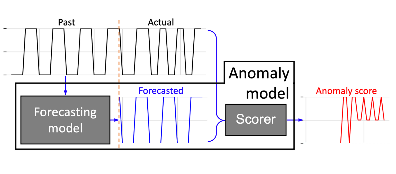
Figure 1. Darts – Anomaly model: The anomaly model is composed of one forecasting model and one or more scorers. The model based on a training or past dataset forecast the time series. The scorer assess and quantified the dissimilarities between the actual and forecasted by assigning anomaly scores to the time series.

In the following demonstration, we use Darts’ LinearRegressionModel (forecasting model) with two different scorers: NormScorer and KMeansScorer. The NormScorer simply returns an element-wise norm of a given order between the data points of the forecasted and actual time series. On the other hand, the KmeansScorer creates an anomaly score time series in multiple steps, including training a k-means model. This scorer applies a moving window on the difference between the forecasted and actual time series, then trains a k-means model on the resulted vectors. For scoring, the KmeansScorer uses the same moving window and returns the distance to the closest of a k centroids for each vector. With an additional post-processing step, these assigned scores are converted to point-wise anomaly scores by taking the mean of the scores of the overlapping windows. The motivation for using window sizes larger than 1 is to enable the detection of contextual anomalies and not only to locate abnormalities for each data point of the time series independently. Furthermore, scorers allow for both component-wise scoring (resulting in two anomaly score time series) or for joint scoring, namely by concatenating the two data points/windows prior to applying the scoring method (as a consequence, the window size required to be defined double in the joint-case).

Anomaly detection use case: arrhythmia detection

In this section, we demonstrate how to use Darts’ anomaly detection module in the healthcare domain. We will set up an anomaly detection model to detect arrhythmia (abnormality of the heart rate) in a publicly available electro-cardiogram (ECG) dataset. The MIT-BIH Supraventricular Arrhythmia Database (SVDB) contains 2 channels, and 78 half-hour ECG recordings obtained from 47 objects between 1975-1979 [7]. A pre-processed version of the SVDB dataset has been created for anomaly detection by Schmidl et al. [8]. Let’s download and unpack the data:

import requests
import zipfile

# Download file from a link
URL = "https://nextcloud.hpi.de/s/tzLZPfcepQgrFrP/download"
response = requests.get(URL)
open("./SVDB.zip", "wb").write(response.content)

# Unzip dataset
with zipfile.ZipFile("./SVDB.zip", 'r') as zip_ref:
zip_ref.extractall("./")

The downloaded CSV file can be directly imported into a TimeSeries – Darts’ native time series data class. The TimeSeries object offers easy-to-use, pandas-like data manipulation for time series.

from darts import TimeSeries

# Load data into darts TimeSeries object
timeseries = TimeSeries.from_csv("./multivariate/SVDB/842.test.csv", time_col='timestamp')
ts_ecg = timeseries[['ECG1','ECG2']]
ts_anomaly = timeseries['is_anomaly']

As each time series is composed of 230400 data points (30 mins data acquisition at 128 Hz), we specify a smaller time frame for better interpretability.

import datetime
import matplotlib.pyplot as plt

# Define start and endpoint of timeseries
end = ts_ecg.get_timestamp_at_point(34560) # Hence, 34560 corresponds to 4.5min at 128Hz

# Plot the data and the anomalies (within the start and end timestamps)
fig, ax = plt.subplots(3, 1)
ts_ecg['ECG1'][:end].plot(ax=ax[0])
ts_ecg['ECG2'][:end].plot(ax=ax[1])
ts_anomaly[start:end].plot(ax=ax[2], label="Known anomalies", color="r")
plt.show()

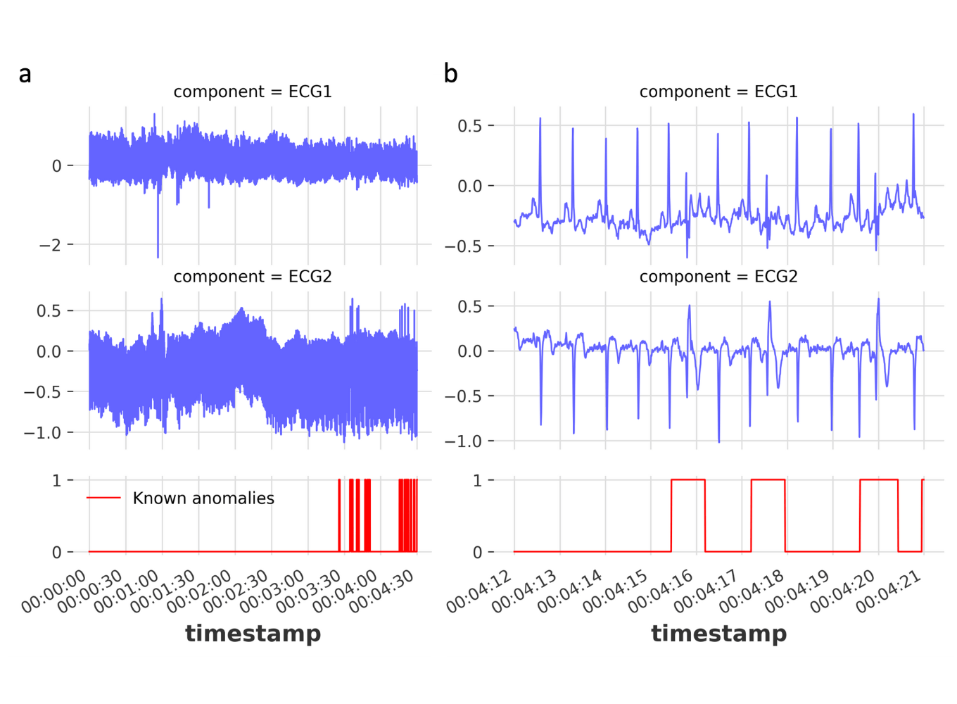
Figure 2. Example ECG signals and corresponding anomalies: (a) The first 5 mins of the two channel ECG signals and corresponding anomalies (top, middle and bottom panels, respectively). (b) Zoomed in time series to showing individual anomalies. The displayed time series are from the dataset 842.test.csv.

We create a train set on which we will train the model, and a test set for model evaluation (for simplicity of this example we skip the validation set). Important is that the training set does not contain any anomalies.

# Create train and test dataset for demonstration
ts_ecg_train = ts_ecg[:25000]
ts_ecg_test = ts_ecg[25000:35000]
ts_anomaly_test = ts_anomaly[25000:35000]

We won’t perform hyper parameter optimization for the model parameters in this example, but rather make some informed guesses.

The 2 channel ECG signal is a periodic signal capturing the polarization and depolarization of the cardiac tissue over time (Figure 2a,b). Despite certain signal drift mainly stemming from the accountable artifacts (e.g., breathing/movement of the patient), the labelled anomalies are mostly frequently shifts (Figure 2b). This frequency shift mostly occurs due to a premature QRS complex (largest spike of each beat) resulting in a fast heart beat followed by an irregular slow one. Since the anomaly is related to the periodicity of the signal, one could set the window size to a multiple of the periodicity of the signal. We can find the periodicity with Darts’s plot_acf function (auto-correlation function, Figure 3).

from darts.utils.statistics import plot_acf

# Visualise signal auto correlation to identify most common periodicity
plot_acf(ts=ts_ecg_train['ECG1'], max_lag=220)
plt.show()

period = 95

In our time series, the auto correlation reveals a peak around period of 90 – therefore with some buffer we will choose 95 as our main signal period.

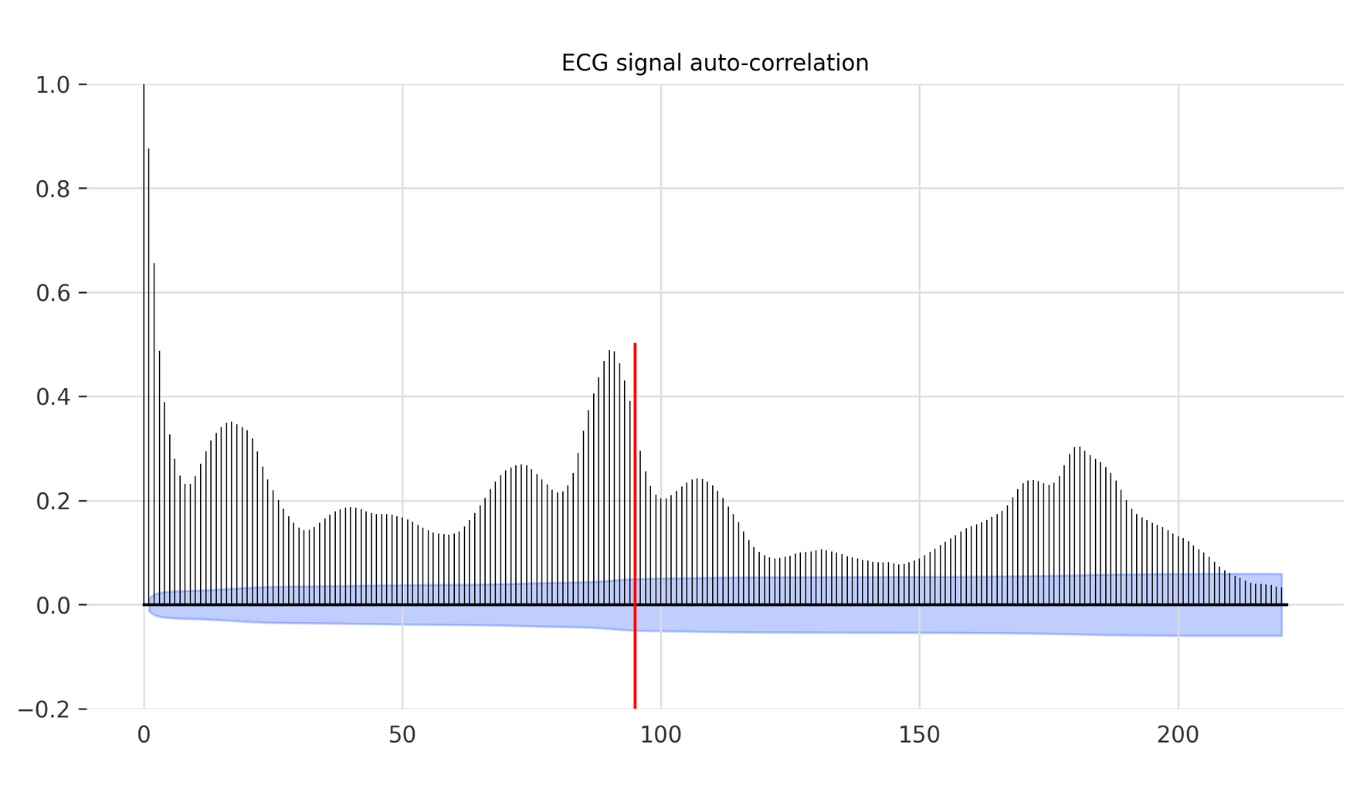
Figure 3. Auto-correlation of an ECG signal. To identify the periodicity of an ECG signal ( most frequent rhythm), auto-correlation function is used. Since the anomalies are mostly frequency shifts choosing the right period for allows the anomaly model to better capture the anomalies. (Red vertical line indicates the chosen period – 95)

We use this period to initialize our LinearRegressionModel and KMeansScorer with their ‘lags’ and ‘window’, respectively. As we use the scorer with a component_wise = False option, we need to take the double of the period, as each generated vector will be double the size of the window due to the concatenation of the two components. In addition, we will set the number of clusters to 50 similarly to the work of Schimdl et al. [8]. To fit the anomaly model, we can define a starting point at which a prediction is computed for a future time. In our example, we set this point to be at the length of two periods.

from darts.metrics import mae, rmse
from darts.models import LinearRegressionModel
from darts.ad.scorers import NormScorer, KMeansScorer
from darts.ad.anomaly_model.forecasting_am import ForecastingAnomalyModel

# Instatiate of a forecasting model - e.g. RegressionModel with a defined lag
forecasting_model = LinearRegressionModel(lags=period)

# Instantiate the anomaly model with: one forecasting model, and one or more scorers (and corresponding parameters)
anomaly_model = ForecastingAnomalyModel(
    model=forecasting_model,
    scorer=[
        NormScorer(ord=1),
        KMeansScorer(k=50, window=2*period, component_wise=False)
    ],
)

# Fit anomaly model
START = 2 * period
anomaly_model.fit(ts_ecg_train, start=START, allow_model_training=True)

After fitting the anomaly model (both the forecasting model and KMeansScorer under the hood), the anomaly model is ready to generate anomaly scores of the defined test time series. To evaluate the forecasting model performance, we assess its performance on the test set by root-mean-square error (MSE) and mean absolute error (MAE).

# Score with the anomaly model (forecasting + scoring)
anomaly_scores, model_forecasting = anomaly_model.score(
    ts_ecg_test, start=2*period, return_model_prediction=True
)

# Compute the MAE and RMSE on the test set
print(f"On testing set -> MAE: {mae(model_forecasting, ts_ecg_test)}, RMSE: {rmse(model_forecasting, ts_ecg_test)}")

Darts comes with an in-built visualization tool for the anomalies along the predicted values of the forecasting models. The method ‘show_values()‘ performs the prediction of the timeseries data and applies the scores on the test and forecasted time series. The performance of the 2 anomaly detection models with different scorers are captured as part of the sub figure titles above the actual anomaly score time series.

# Visualize anomalies
anomaly_model.show_anomalies(
    series=ts_ecg_test,
    actual_anomalies=ts_anomaly_test,
    start=START,
    metric="AUC_ROC",
)
plt.show()

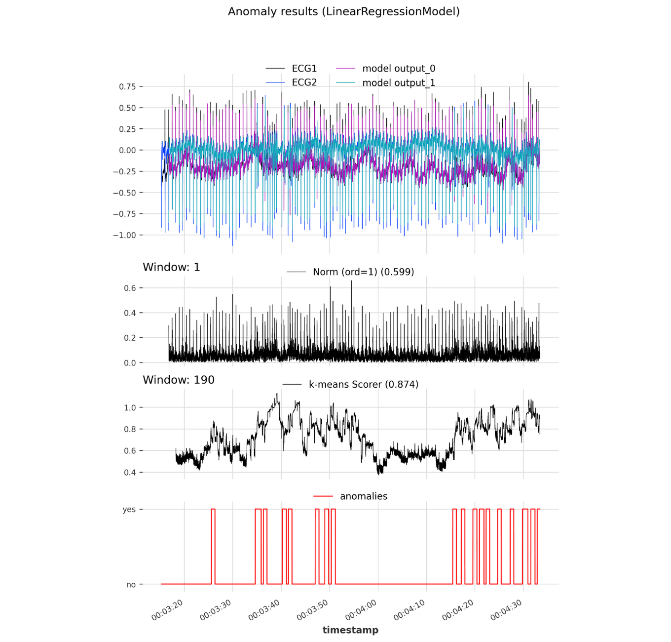
Figure 4. Darts anomaly model: Anomaly results of a developed Darts anomaly model instantiated with a LinearRegressionModel and two scorers: NormScorer and KMeansScorer. Top panel shows both ECG signal as well as corresponding forecasted time series. The middle panels show the anomaly scores and evaluted AUC-ROC performance of the Norm and KMeans scorer. The bottom panel contains the actual anomalies.

The NormScorer achieved a moderate performance of 0.599 AUC-ROC. Analyzing the anomaly score time series shows that the NormScorer scores higher at the heart-beat peaks in one cardiac period, as the forecasting model tends to have lower accuracy at these points (Figure 4). In comparison, the KMeansScorer achieved better results with an AUC-ROC of 0.874 on the given test ECG dataset. This scorer, by evaluating patterns instead of simply point-wise comparing the actual and predicted dataset, able to capture contextual anomalies. As a result, the KMeansScorer effectively identifies anomalous patterns by evaluating how dissimilar they are to typical patterns observed in the training set. Therefore, less common irregularities receive high anomaly scores (Figure 4), which translates into increased sensitivity for detecting arrhythmia.

Concluding remarks

To sum up, we showed how to use Darts for time series data analysis and manipulation, and how to create, train, and evaluate an anomaly model with the new anomaly detection module. And this all in under 50 lines of code! The model used a LinearRegressionModel with 2 different scorers to identify arrhythmia captured by 2 channel ECG measurements of a patient.

Time series analysis is a valuable tool for gaining insights into the patterns and trends so inherent in healthcare data, the robust and convenient interface of Darts lowers the barrier of time series analysis, and the recent addition of the anomaly detection module opens up new possibilities for quickly prototyping solutions in the healthcare space.

References

[1] Agliari, E., Barra, A., Barra, O.A. et al. Detecting cardiac pathologies via machine learning on heart-rate variability time series and related markers. Sci Rep 10, 8845 (2020).

[2] Sander Dijkstra, Stef Baas, Aleida Braaksma, Richard J. Boucherie, Dynamic fair balancing of COVID-19 patients over hospitals based on forecasts of bed occupancy, Omega, Volume 116, 2023, 102801, ISSN 0305-0483

[3] Dijkstra S, Baas S, Braaksma A, Boucherie RJ. Dynamic fair balancing of COVID-19 patients over hospitals based on forecasts of bed occupancy. Omega. 2023 Apr;116:102801

[4] Li Shao, Rui Xue, Xiaoyan Lu, Jie Liao, Xin Shao, Xiaohui Fan, Identify differential genes and cell subclusters from time-series scRNA-seq data using scTITANS, Computational and Structural Biotechnology Journal, Volume 19, 2021, Pages 4132-4141, ISSN 2001-0370

[5] Deutsch T, Lehmann ED, Carson ER, Roudsari AV, Hopkins KD, Sönksen PH. Time series analysis and control of blood glucose levels in diabetic patients. Comput Methods Programs Biomed. 1994 Jan;41(3-4):167-82

[6] Herzen, Julien & Lässig, Francesco & Piazzetta, Samuele & Neuer, Thomas & Tafti, Léo & Raille, Guillaume & Van Pottelbergh, Tomas & Pasieka, Marek & Skrodzki, Andrzej & Huguenin, Nicolas & Dumonal, Maxime & Kościsz, Jan & Bader, Dennis & Gusset, Frédérick & Benheddi, Mounir & Williamson, Camila & Kosinski, Michal & Petrik, Matej & Grosch, Gaël. (2021). Darts: User-Friendly Modern Machine Learning for Time Series.

[7] Goldberger, A., Amaral, L., Glass, L., Hausdorff, J., Ivanov, P. C., Mark, R., … & Stanley, H. E. (2000). PhysioBank, PhysioToolkit, and PhysioNet: Components of a new research resource for complex physiologic signals. Circulation [Online]. 101 (23), pp. e215–e220.

[8] Sebastian Schmidl, Phillip Wenig, and Thorsten Papenbrock. Anomaly Detection in Time Series: A Comprehensive Evaluation. PVLDB, 15(9): 1779 – 1797, 2022. doi:10.14778/3538598.3538602